Mathematical Modelling Questions And Answers Pdf

Consider a linear time-invariant system whose input r(t) and output y(t) are related by the following differential equation:

\(\frac{{{d^2}y\left( t \right)}}{{d{t^2}}} + 4y\left( t \right) = 6r\left( t \right)\)

The poles of this system are at

1. +2j, -2j
2. +2, -2
3. +4, -4
4. +4j, -4j

Answer (Detailed Solution Below)

Option 1 : +2j, -2j

Concept:

A transfer function is defined as the ratio of Laplace transform of the output to the Laplace transform of the input by assuming initial conditions are zero.

TF = L[output]/L[input]

\(TF = \frac{{C\left( s \right)}}{{R\left( s \right)}}\)

For unit impulse input i.e. r(t) = δ(t)

⇒ R(s) = δ(s) = 1

Now transfer function = C(s)

Therefore, the transfer function is also known as the impulse response of the system.

Transfer function = L[IR]

IR = L-1 [TF]

Calculation:

Given the differential equation is,

\(\frac{{{d^2}y\left( t \right)}}{{d{t^2}}} + 4y\left( t \right) = 6r\left( t \right)\)

By applying the Laplace transform,

s² Y(s) + 4 Y(s) = 6 R(s)

\( \Rightarrow \frac{{Y\left( s \right)}}{{R\left( s \right)}} = \frac{6}{{{s^2} + 4}}\)

Poles are the roots of the denominator in the transfer function.

⇒ s² + 4 = 0

⇒ s = ±2j

Which of the following modelling methods uses Boolean operations?

1. Boundary representation
2. Constructive solid geometry
3. Surface modelling
4. Wireframe modelling

Answer (Detailed Solution Below)

Option 2 : Constructive solid geometry

Explanation:

• Boolean operation is an important way in geometry modeling.
• It is the main way to build a complex model from simple models, and it is widely used in computer-aided geometry design and computer graphics.
• Traditional Boolean operation is mainly used in solid modeling to build a complex solid from primary solid e.g. cube, column, cone, sphere, etc.
• With the development of computer applications, there are many ways to represent digital models, such as parametric surface, meshes, point model, etc.
• Models become more and more complex, and features on models such as on statutary artworks are more detailed.

Let a causal LTI system be characterized by the following differential equation, with initial rest condition

\(\frac{{{d^2}y}}{{d{t^2}}} + 7\frac{{dy}}{{dt}} + 10y\left( t \right) = 4x\left( t \right) + 5\frac{{dx\left( t \right)}}{{dt}}\)

where x(t) and y(t) are the input and output respectively. The impulse response of the system is (u(t) is the unit step function)

1. 2e^-2tu(t) – 7 e^-5tu(t)
2. –2e^-2tu(t) + 7 e^-5tu(t)
3. 7e^-2tu(t) – 2 e^-5tu(t)
4. –7e^-2tu(t) + 2 e^-5tu(t)

Answer (Detailed Solution Below)

Option 2 : –2e^-2tu(t) + 7 e^-5tu(t)

\(\frac{{{d^2}y}}{{d{t^2}}} + 7\frac{{dy}}{{dt}} + 10y\left( t \right) = 4x\left( t \right) + 5\frac{{dx}}{{dt}}\)

Apply Laplace transform on both sides,

s²Y(s) + 7sY(s) + 10Y(s) = 4 X(s) + 5s X(s)

⇒ (s² + 7s + 10) Y(s) = (4 + 5s) X(s)

\(\Rightarrow \frac{{Y\left( s \right)}}{{X\left( s \right)}} = \frac{{\left( {4 + 5s} \right)}}{{{s^2} + 7s + 10}}\)

\(\Rightarrow \frac{{Y\left( s \right)}}{{X\left( s \right)}} = \frac{{4 + 5s}}{{\left( {s + 5} \right)\left( {s + 2} \right)}} = \frac{7}{{\left( {s + 5} \right)}} - \frac{2}{{\left( {s + 2} \right)}}\)

Apply inverse laplace transform

⇒ y(t) = 7e^-5tu(t) – 2e^-2t u(t)

For a tachometer, ie θ(t) is the an rotor displacement in radians, e(t) is the output voltage and k_t is the tachometer constant in V/rad/sec, then the transfer function \(\frac{{E\left( S \right)}}{{\theta\left( S \right)}}\) will be:

1. K_ts²
2. \(\frac{{k_t}}{s}\)
3. K_ts
4. K_t

Answer (Detailed Solution Below)

Option 3 : K_ts

Output = e(t)

Input =  (t)

\({\rm{e}}\left( {\rm{t}} \right) \propto \frac{{{\rm{d\theta }}\left( {\rm{t}} \right)}}{{{\rm{dt}}}}\)

Taking LT,

E(s) = K_ts θ(s)

\(\Rightarrow {\rm{TF}} = \frac{{E\left( S \right)}}{{\theta\left( S \right)}} = {{\rm{k}}_t}s\)

The mechanical system shown in the figure below has its pole(s) at:

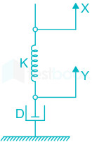
1. -K/D
2. -D/K
3. -DK
4. 0, -K/D

Answer (Detailed Solution Below)

Option 1 : -K/D

Concept:

Damping force:

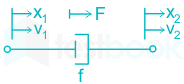
\(F = f\frac{{d\left( {{x_1} - {x_2}} \right)}}{{dt}} = f\left( {{v_1} - {v_2}} \right)\)

F: Damper force

f: Damper constant

x₁, x₂: Displacement at side 1 and side 2 of the damper

v₁, v₂: Velocity at side 1 and side 2

Spring force

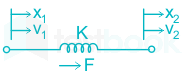
\(F = k\left( {{x_1} - {x_2}} \right) = k\mathop \smallint \nolimits \left( {{v_1} - {v_2}} \right)dt\)

k: Spring constant

Calculation:

Method 1:

Given damper constant is D and the Spring constant is k

Assuming that velocities at side 1 and 2

K ∫(y - x) dt + D (y – 0) = 0

Dy +k ∫ y dt – k ∫ x dt = 0

Applying the Laplace Transform

\(DY\left( s \right) + \frac{k}{s}Y\left( s \right) - \frac{k}{s}X\left( s \right) = 0\)

\(Y\left( s \right)\left[ {\frac{{Ds + k}}{s}} \right] = \frac{k}{s}X\left( s \right)\)

\(\frac{{Y\left( s \right)}}{{X\left( s \right)}} = \frac{k}{{Ds + k}}\)

Pole is present at s = - k / D

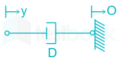
Method 2:

Given damper constant is D and the Spring constant is k

Assuming displacement at side 1 and 2

\(k\left( {y - x} \right) + D\frac{{d\left( {y - 0} \right)}}{{dt}} = 0\)

Applying the Laplace Transform

k Y(s) – k X(s) + D sY(s) = 0

Y(s) (k + Ds) – k X(s) = 0

\(\frac{{Y\left( s \right)}}{{X\left( s \right)}} = \frac{k}{{Ds + k}}\)

Pole is present at s = - k / D

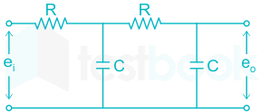
The transfer function of the network shown above is

1. \(\frac{1}{{{s^2}{T^2} + 2sT + 1}}\)
2. \(\frac{1}{{{s^2}{T^2} + 3sT + 1}}\)
3. \(\frac{1}{{{s^2}{T^2} + sT + 1}}\)
4. \(\frac{1}{{{s^2}{T^2} + 1}}\)

Answer (Detailed Solution Below)

Option 2 : \(\frac{1}{{{s^2}{T^2} + 3sT + 1}}\)

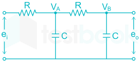
By applying KCL at node A,

\(\frac{{{V_A} - {e_i}}}{R} + \frac{{{V_A} - {V_B}}}{R} + \frac{{{V_R}}}{{{X_C}}} = 0\)

\(\Rightarrow {V_A}\left[ {\frac{2}{R} + \frac{1}{{{X_C}}}} \right] - \frac{{{e_i}}}{R} - \frac{{{V_B}}}{R} = 0\)      …1)

By applying KCL at node B,

\(\frac{{{V_B} - {V_A}}}{R} + \frac{{{V_B}}}{{{X_c}}} = 0\)

\({V_B}\left[ {\frac{1}{R} + \frac{1}{{{X_c}}}} \right] = \frac{{{V_A}}}{R} \Rightarrow {V_A} = {V_B}\left[ {1 + \frac{R}{{{X_c}}}} \right]\)     …2)

From equation 1) and 2)-

\( \Rightarrow {V_B}\left[ {1 + \frac{R}{{{X_C}}}} \right]\left[ {\frac{2}{R} + \frac{1}{{{X_c}}}} \right] - \frac{{{V_B}}}{R} = \frac{{{e_i}}}{R}\)

\( \Rightarrow {V_B}\left[ {\frac{2}{R} + \frac{1}{{{X_c}}} + \frac{2}{{{X_c}}} + \frac{R}{{X_c^2}} - \frac{1}{R}} \right] = \frac{{{e_i}}}{R}\)      …3)

As we can see from the circuit diagram, V_B = e₀

\( \Rightarrow {e_0}\left[ {\frac{1}{R} + \frac{3}{{{X_c}}} + \frac{R}{{X_c^2}}} \right] = \frac{{{e_i}}}{R}\)

\(\Rightarrow \frac{{{e_0}}}{{{e_i}}} = \frac{1}{{R\left[ {\frac{1}{R} + \frac{3}{{{X_c}}} + \frac{R}{{X_c^2}}} \right]}}\)

\(= \frac{1}{{{{\left( {CsR} \right)}^2} + 3RCs + 1}}\)

Time constant, T = RC

\(h\left( T \right) = \frac{1}{{{T^2}{s^2} + 3Ts + 1}}\)

Which one of the following statements related to modeling of system dynamics is NOT true?

1. The transfer function is not changed by a linear transformation of state
2. A given state description can be transformed to a controllable canonical form if the controllability matrix is nonsingular
3. A change of state by a nonsingular linear transformation does not change the
4. Zeros cannot be computed from its state description matrices

Answer (Detailed Solution Below)

Option 3 : A change of state by a nonsingular linear transformation does not change the

Modeling of Dynamic System:

• A dynamic system is a kind of system whose behavior is a function of time.
• Static system analysis does not give an accurate analysis while Dynamic system analysis does give an accurate analysis.
• Example: An aircraft is subjected to time-varying stress during the flight through turbulent air hard landing is an example of a Dynamic system.
• Dynamic system analysis is more complex than static system analysis since the conclusion based on static system analysis is not correct.
• In the dynamic system, the transfer function does not change by a linear transformation of the state.
• The dynamic modeling starts with the physical component description of the system's understanding of component behavior to create the mathematical model.
• A given state description in the mathematical model can be transformed to a controllable canonical form if the controllability matrix is non-singular. And zero cannot be computed from this matrix.

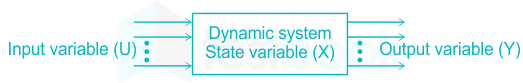
​The dynamic system state variable is used for:

• Analysis, Identification, and Synthesis of Dynamic System.
• Predict the future behavior (Y) of the system when subjected to future input variables (U) and present (X).

The transfer function of tachometer is of the form

1. \(\frac{K}{{s\left( {s + 1} \right)}}\)

2. \(\frac{K}{{\left( {s + 1} \right)}}\)

3. \(\frac{K}{s}\)

4. K.s

Answer (Detailed Solution Below)

Output = e(t)

Input = (t)

\({\rm{e}}\left( {\rm{t}} \right) \propto \frac{{{\rm{d\theta }}\left( {\rm{t}} \right)}}{{{\rm{dt}}}}\)

Taking LT,

E(s) = Kts θ(s)

\(\Rightarrow {\rm{TF}} = \frac{{E\left( S \right)}}{{\theta\left( S \right)}} = {{\rm{k}}_t}s\)

Mathematical Modeling and Representation of Systems MCQ Question 9:

Consider a linear time-invariant system whose input r(t) and output y(t) are related by the following differential equation:

\(\frac{{{d^2}y\left( t \right)}}{{d{t^2}}} + 4y\left( t \right) = 6r\left( t \right)\)

The poles of this system are at

1. +2j, -2j
2. +2, -2
3. +4, -4
4. +4j, -4j

Answer (Detailed Solution Below)

Option 1 : +2j, -2j

Concept:

A transfer function is defined as the ratio of Laplace transform of the output to the Laplace transform of the input by assuming initial conditions are zero.

TF = L[output]/L[input]

\(TF = \frac{{C\left( s \right)}}{{R\left( s \right)}}\)

For unit impulse input i.e. r(t) = δ(t)

⇒ R(s) = δ(s) = 1

Now transfer function = C(s)

Therefore, the transfer function is also known as the impulse response of the system.

Transfer function = L[IR]

IR = L-1 [TF]

Calculation:

Given the differential equation is,

\(\frac{{{d^2}y\left( t \right)}}{{d{t^2}}} + 4y\left( t \right) = 6r\left( t \right)\)

By applying the Laplace transform,

s² Y(s) + 4 Y(s) = 6 R(s)

\( \Rightarrow \frac{{Y\left( s \right)}}{{R\left( s \right)}} = \frac{6}{{{s^2} + 4}}\)

Poles are the roots of the denominator in the transfer function.

⇒ s² + 4 = 0

⇒ s = ±2j

Mathematical Modeling and Representation of Systems MCQ Question 10:

For the system given figure, e(t) is the error between input x(t) and output y(t)

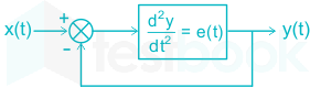
If x(t) = u(t) and all the initial conditions are zero, then e(t) will be

1. –sin t
2. –cos t
3. sin t
4. cos t

Answer (Detailed Solution Below)

Option 4 : cos t

From the block diagram,

e(t) = -y(t) + x(t)

\(\Rightarrow \frac{{{d^2}y}}{{d{t^2}}} = - y\left( t \right) + x\left( t \right)\)

\(\Rightarrow \frac{{{d^2}y}}{{d{t^2}}} = - y\left( t \right) + u\left( t \right)\)

By applying Laplace transform,

\(\Rightarrow {s^2}y\left( s \right) = - y\left( s \right) + \frac{1}{s}\)

\(\Rightarrow y\left( s \right) = \frac{1}{{s\left( {1 + {s^2}} \right)}}\)

\(e\left( t \right) = \frac{{{d^2}y}}{{d{t^2}}}\)

⇒ E(s) = s² y(s)

\(\Rightarrow E\left( s \right) = {s^2} \times \frac{1}{{s\left( {1 + {s^2}} \right)}} = \frac{s}{{1 + {s^2}}}\)

By applying inverse Laplace transform,

⇒ e(t) = cos t

Mathematical Modelling Questions And Answers Pdf

Source: https://testbook.com/objective-questions/mcq-on-mathematical-modeling-and-representation-of-system--5eea6a1039140f30f369e947

Posted by: stanleygrou1963.blogspot.com

Share this post